Photovoltaic (PV) Panel - Performance Modelling 

In an earlier note on the site [Photovoltaic (PV) - Electrical Calculations], the theory of solar (PV) cell calculations was introduced.  In particular the post looked at the PV cell equivalent circuit and the electrical characteristics of the cell.  This note expands on the previous post and shows how we can use tools like MatLab to model the performance of a complete solar panel.

Definitions:

• Solar cell - the basic semiconductor device to convert light to electricity
• PV module - several solar cells in series and parallel to form practically usable size
• PV panel - a collection of one or more modules, wired together and forming a commercial product
• PV array - an installation of several PV panels, generating usable electricity

Note: terms are often used differently, although it is usually easy to determine what is what from the context.

Modelling the PV Panel

A commercially available product for which manufacturers construction and performance data is available to illustrate the process of modelling a PV panel.  We then build a model of this PV panel and compare the predicted results from the model with the manufacturers data.

As an example, I randomly chose a panel for a reputable manufacturer (where there is a datasheet available).  The panel is a Canadian SolarCS6P polycrystalline produce (255P module) with a nominal power output of 255 W.   You can find a link to the datasheet at the bottom of the note.

There are several programs that can be uses to model a PV systems; this note used MatLab Simulink.  The software's SimElectronics module contains ready built a solar cell source which is ideal for our purpose.  Once a model of the panel is built, using MatLab will be able us to integrate this is various energy storage system and power distribution models at a later stage.

The implementation of the solar cell follows closely this equivalent circuit shown in  the exception of using two diodes.  The second diode can provide a more accurate model (although for this example, I did not try and optimise any parameters for the second diode).

The implementation of the solar cell follows the equivalent circuit as shown in our [Photovoltaic (PV) - Electrical Calculations note], with the exception of using two diodes not one.  The second diode can provide a more accurate model (although, for this example, I did not try and optimise any parameters for the second diode).

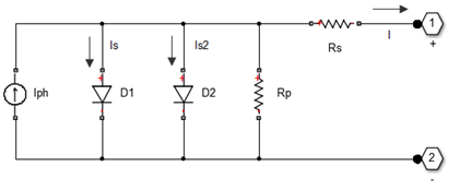PV Cell Equivalent Circuit (two diodes)

*click on images to view larger versions

Finding Parameters

The first step in building our PV model is to estimate the solar cell parameters from the data sheet. 

The basic idea is to build a model of the cell (using the SimElectronics solar cell source block).  The MatLab function 'fminsearch' is then used to optimize the model parameters (by iteration) to so that the generated results match the data sheet curves.   The I-V curve for 1000 w/m2 is first optimized using the iterative procedure, followed by the temperature dependencies.

Note: the data file for optimisation was created by taking the points directly from I-V temperature curves given in the data sheet.  WebPlotDigitizer was used to do digitize the curves;  a free great on-line tool.

Running my data through the optimisation procedure, yielded:

• Optimized parameters for the solar cell main dialog tab
  • Diode saturation current, I_s = 2.7098e^-10 A
  • Solar generated current, I_ph = 9.0012 A
  • Quality factor, ec = 1.0
  • Series resistance, R_s = 0.0056
  • Parallel resistance, R_p = 39 MΩ
• Optimized parameters for the solar cell temperature dialog tab
  • First order temperature coefficient, TIPH1 = 0.001 K^-1
  • Energy gap, EG = 1.2593 eV
  • Diode temperature exponent,  TXIS1 = 1.7109e^-07
  • Series resistor temperature exponent = 2.376e^-07
  • Parallel resistor temperature exponent = 0.3093

Note: it took a few days to get this working – there were issues with digitized data numbers of iterations and which model parameters to vary.  In the end though, it does work, and we do end up with a good model of the cell.

Resultant PV Panel Model

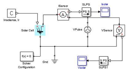Solar Cell Model (MatLab)

The model is quite simple.  The Solar Cell is the main component and has been set with the optimized parameters derived above.  The number of series cells is set to 60 (obtained from the manufacturers data sheet).  If you want more information on how the solar cell block works, you can visit pulse generator ramps the voltage up from zero to 40, allowing us to produce the I-V curves (and power by multiplying the voltage and current).  The model output taken vie the two scopes.

The model is quite simple.  The Solar Cell is the main component and has configured with the optimized parameters derived above.  The number of series cells is set to 60 (obtained from the manufacturers data sheet).  If you want find out more on how the solar cell block works, you can visit the MatLab Solar Cell Documentation.  The voltage pulse generator ramps the voltage up from zero to 40, allowing us to produce the I-V curves (and power by multiplying the voltage and current).  The model output taken vie the two scopes.

To verify that the model is working correctly, I used a script that iterates through various irradiance and temperatures to produce the following curves.  Irradiance and temperature values have been chosen to be the same as those in the manufacturers data sheet to enable direct comparisons.

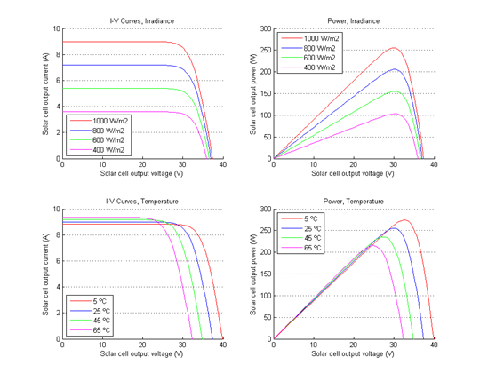IV and Power Curves for varying irradiance and temperature

The first chart shows IV curves for different levels of irradiance. These curves when compared to those in the datasheet and are seen to be a very good match.  Power curves (not shown on the manufacturer's data sheet) are also plotted (for various irradiance).   The power curves show the anticipated maximum power point and show that the effect irradiance on it's position (maximum power point voltage) is limited.

The next chart shows the IV and power curves for different temperatures.  Again the IV curves follow those shown on the manufacturers data sheet. In addition, the power curves clearly illustrate how the maximum power point moves and changes in magnitude as the temperature changes. 

From the above, it is seen that we now have a good model for the PV panel and can utilise this in any future studies.

Application Examples

Now that we have an accurate model for our PV panel, it is now possible to expand this to deal with real life situations.  We can connect several panels in series and parallel to build large arrays.  We can add in energy storage mechanisms and investigate how these work.  Alternatively we can add inverters, connect this to our power system and see how a PV array affects power flow, voltage levels or system harmonics.

To illustrate using the model, I kept the following examples simple, and yet, hopefully, practical and useful. 

Example 1

Intuitively PV systems would perform better in sunnier climates.  However, sunnier climates tend to be hotter, and the increase in temperature reduces the output of any PV system. 

As an example, I did hope to do this exercise over several locations, but there is a cost for data.  For demonstration, I decided to use the example data file from Meteonorm, which contains a full year of hourly data for Bern in Switzerland.  For other locations, data could be purchased if required.

By writing a script, we can iterate through each hourly piece of data and calculate the energy obtained during that hour. We can then sum these to obtain to total annual energy output.  In finding the power for each iteration, I determined the maximum power point (simulating maximum power point tracking, MPPT) and used that value in the annual summation. 

As a benchmarking exercise, four sets of calculation were performed - for the STC temperature of 25 ºC, using the actual hourly temperature, using the average yearly temperature and using the average monthly temperature. 

The simulation results are (Annual Maximum Power Output (kW) - Bern, Switzerland):

* the per unit [pu] values take the STP calculation as baseline.

While the annual energy in kW.hr gives us the actual figures, it is useful to look at the per unit comparisons.  Using the actual temperatures (which are typically lower than 25 ºC in Bern), shows that we can expect the PV panel to perform 3% better than indicated by the STC temperature conditions.  Using average yearly or monthly temperatures introduces additional errors in the order of 2%.

Note: the figures calculated are the theoretical maximum possible power output.  For instance, the calculation does not take into account, solar panel inclinations, shading, environmental conditions that could reduce the irradiance, inefficient (or no) MPPT, system losses, etc.  If required, these could be integrated into the analysis.

Example 2

Another quick example is to investigate the use of diodes in PV panel arrays.  For this example, I connected to parallel strings of four panels each in strings. Using datasheet information, this should give us approximately 120 V,  at 16.8 A or approximately 2 kW (at 1000 w/m² and 25 ºC).  A resistor of 7Ω  and small inductance of 10 mH is used as the test load. 

PV Array (no diodes)

The circuits and results of the simulation are:

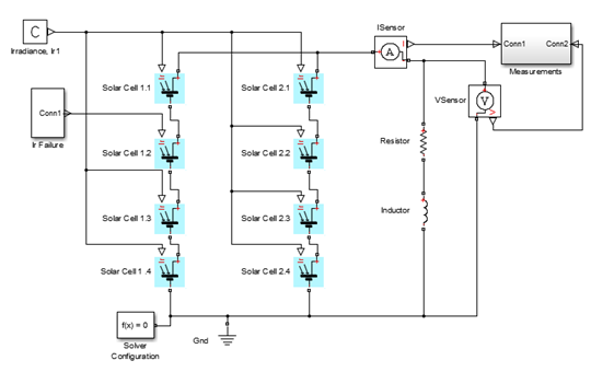PV Array (no diodes)

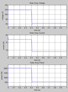PV Array (no diodes) - results

After 0.4 S, the irradiance on panel 1.2 is reduced from 1000 w/m2 to zero (simulating shading or something wrong with the cell).  As array 1.2 now starts to absorb power, the output voltage and power of the full array drop.  The voltage drops from 120 V to just over 60 V.  Available current decreases and the power drops for 2 kW to just over 500 W.

PV Array (diodes)

Two types of diode are commonly used with PV arrays - blocking and bypass.  Blocking diodes are placed between strings and in the array output.  The function of blocking diodes is to stop any back-feed of power from adjacent strings, connected energy storage or grid connections.

Bypass diodes are placed in parallel with the PV modules.  Normally the diode resistance is higher than that of the PV panel and current flows (and is generated) through the panel.  When the irradiance drops, the panel impedance increases and current flows through the diode rather than the panel (stopping the panel absorbing power).

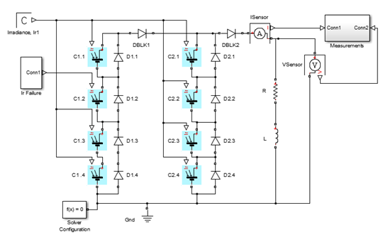PV Array (diodes)

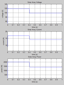PV Array (diodes) - results

The above diagrams show the simulation complete with diodes.  There is a marked improvement in both output voltage and power delivered.  In this example, the available is nearly three times that of a system without diodes.   In addition, the diode limits the voltage across the panel avoiding large losses within the panel which would cause heat and damage.

Summary

Standard solar modelling software is normally the starting point for any design.  However, having the ability to model PV systems in programs like MatLab, allow us to go beyond any constraints with standard software.  Taking a solar powered car for example; it is unlikely this could be modelled using any purposely built solar software on the market.  However, within MatLab we could model the solar panels, drive chain, energy storage and regenerative systems and tie this into the actual travel of the car between locations.  Another example would be using a MatLab simulation of a large PV array in conjunction with the power system model to look at harmonic, voltage drop and transient inrush issues. 

By using MatLab, we can model a PV system as part of a larger dynamic system.  We can used these models to develop specific studies to investigate almost any aspect of the system performance.

Attachments

Canadian Solar CS6P polycrystalline panel datasheet